The History of Logit

Logit

Author

Pingfan Hu

Published

May 20, 2024

Useful Links

Research Paper	The Origins of Logit Regression
Lecture Slides	Intro to Choice Modeling
Online Article	What is Logit (Chinese)

Abstract

This blog describes a brief history of the Logit Model.

It starts from the famous Malthus population problem, and explains the necessity of transforming from probability to logit.

The Malthus Population Problem

1. The Malthusian Growth Model

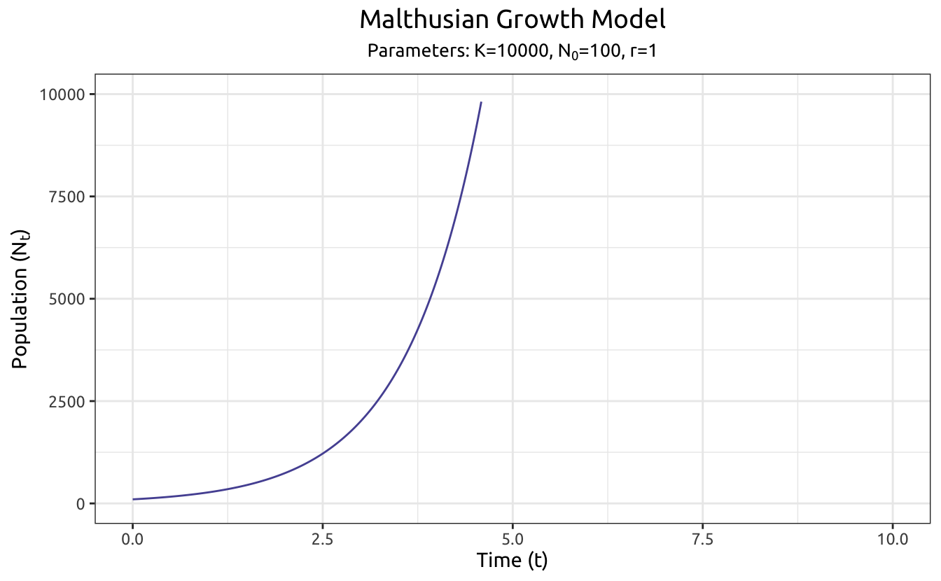
In the biology class of my high school, I learned that the population will grow exponentially given unlimited resources and spaces. This is called the “Malthus Population Problem” and was give the name “J Curve”, since the exponential Malthusian Model looks like the English letter J.

The Malthusian Growth Function:

\[ N_t = N_0 \cdot e^{rt} \] Where:

$K$ (not in this equation but will be used later) stands for the carrying capacity, which is the maximum allowed population in the system.
$N_t$ stands for the population size at time of $t$,
$N_0$ stands for the initial population size, and
$r$ stands for the growth rate.

The Malthusian Growth Model (CDF):

Code

# Parameters
K <- 10000
N_0 <- 100
r <- 1

# Calculation
x <- seq(0, 10, length.out = 400)
N_t_malthus <- N_0 * exp(r * x)
data_malthus <- data.frame(Time = x, Population = N_t_malthus)

# Plotting
ggplot(data_malthus, aes(x = Time, y = Population)) +
  geom_line(color = "#5654A2") +
  labs(title = "Malthusian Growth Model",
       subtitle = expression(
         paste("Parameters: ", K, "=10000, ", N[0], "=100, ", r, "=1")
         ),
       x = "Time (t)",
       y = expression(paste("Population (", N[t], ")"))) +
  ylim(0, 10000) +
  theme_bw(base_family = 'Ubuntu') +
  theme(plot.subtitle = element_text(hjust = 0.5, size = 10),
        plot.title = element_text(hjust = 0.5, size = 14))

In this model, we set a simple scenario of $K$ = 10,000, $N_0$ = 100, and $r$ = 1. It can be seen that the population grows so fast, that it reaches the cap while $t$ value is a little over 4.

2. The Logistic Growth Model

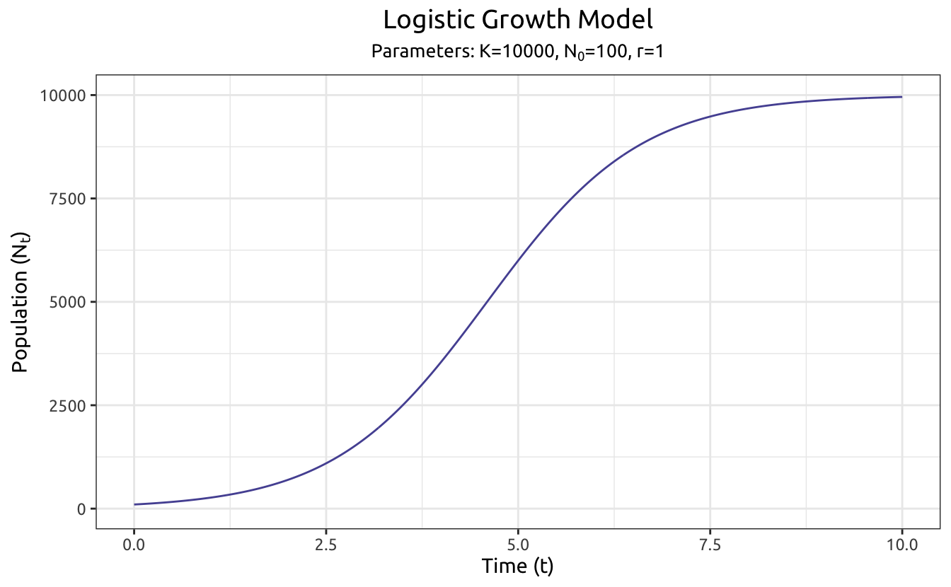
However, this exponential model is unrealistic due to the scarcity of resources and spaces. A Belgian mathematician named Verhulst realized the cap of population growth. He used an S curve to explain this cap. This S curve is perhaps the first S-shaped curve that we could learn in our textbooks.

Verhulst named this distribution “logistique”, originated from a French word “logis”, meaning “lodging” in English. However, we used the word “Logistic” instead for statistical analysis. This model is thus called the “Logistic Model”, or “Logit Model”.

The word “logit” is a portmanteau, coming from logistic + unit.

The Logit Growth Function:

\[ N_t = \frac{K}{1 + \left( \frac{K - N_0}{N_0} \right) e^{-rt}} \]

The Logit Growth Model (CDF):

Code

# Calculation for Logistic Growth Model
N_t_logit <- K / (1 + ((K - N_0) / N_0) * exp(-r * x))
data_logit <- data.frame(Time = x, Population = N_t_logit)

# Plotting the Logistic Growth Model
ggplot(data_logit, aes(x = Time, y = Population)) +
  geom_line(color = "#5654A2") +
  labs(title = "Logistic Growth Model",
       subtitle = expression(
         paste("Parameters: ", K, "=10000, ", N[0], "=100, ", r, "=1")
         ),
       x = "Time (t)",
       y = expression(paste("Population (", N[t], ")"))) +
  ylim(0, 10000) +
  theme_bw(base_family = 'Ubuntu') +
  theme(plot.subtitle = element_text(hjust = 0.5, size = 10),
        plot.title = element_text(hjust = 0.5, size = 14))

This is the “S Curve” we’ve been seen in a lot of scenarios where there is a designed cap of population due to resource scarcity. There are also other S shaped curves. To avoid ambiguity, we use the term “Logit” instead.

The CDF of logit model is an S curve. With a visible diminishing of returns, it is a perfect model for human behavior studies for the purpose of generating a feasible marketing strategy.

The Logit Model

1. Probability vs Logit

The traditional way of defining the probability is to calculate the utility of choosing over the sum of utilities. The equation is written like this:

\[ P_j = \frac{v_j}{v_j + v_k} \]

In this equation, the probability of choosing $j$ over $k$ is the utility of $j$ over the sum of utilities. In this model, utilities are normally distributed.

An alternative way is to use the Logit Model, where we take the logarithm of the odds:

\[ P_j = \frac{e^{v_j}}{e^{v_j} + e^{v_k}} \]

This is again the probability of choosing $j$ over $k$. To generalize the equation, the probability of choosing $j$ over all other alternatives is written as this:

\[ P_j = \frac{e^{v_j}}{\sum_{k=1}^{J} e^{v_k}} \]

The logit model utilizes the Type 1 Extreme Value distribution, and requires independent errors (IIA).

IIA can be problematic when products are close substitutes. For example, in a DCM scenario, alternatives of Taxi, Red Bus, and Blue Bus are in fact 2 alternatives, since the Red Bus and the Blue Bus should be identical and only considered as one alternative. This is ignored by the IIA property.

2. Why Logit

So, why using Logit Model? Why bother transforming the simple probability value into a somewhat non-intuitive value? An important reason is that the Logit Model does not have lower and upper limits. This can be better explained by the Logit Transformation:

\[ \text{Probability} \rightarrow \text{Odds} \rightarrow \text{Logit} \]

In statistics, both probability and odds are used to describe the likelihood of an event occurring, but they have an important difference:

Probability refers to the ratio of the number of times an event A occurs to the total number of possible outcomes, while
Odds refers to the ratio of the probability of an event occurring to the probability of the event not occurring.

The probability equation writes:

\[ P(A) = \frac{\text{Number of Event A}}{\text{Total Number of Events}} \]

The probability $P$ is a real number between 0 and 1. $P = 0$ indicates that an event will definitely not occur, while $P = 1$ indicates that an event will definitely occur. In the case of rolling a die, the probability of rolling a 6 is:

\[ P = \frac{1}{6} \]

The odds equation writes:

\[ \text{Odds} = \frac{\text{Probability of event}}{\text{Probability of no event}} = \frac{P}{1 - P} \]

Continuing with the example of rolling a die, the probability of rolling a 6 is $P = \frac{1}{6}$, and the probability of rolling any other number is $1 - P = \frac{5}{6}$. According to the equation, the odds of rolling a 6 is:

\[ \text{Odds} = \frac{1/6}{5/6} = \frac{1}{5} \]

Now you can see: The ratio of the probability of successfully rolling a 6 to that of not is 1:5.

Like many other concepts in probability theory, the idea of odds originates from gambling. Suppose two people, A and B, bet on rolling a die; if A bets 1 dollar on rolling a 6, B would need to bet 5 dollars to ensure a fair game.

$1/6$ and $1/5$ is not a big difference, but the point is to show that probability is happening vs all, while odds is happening vs not happening.

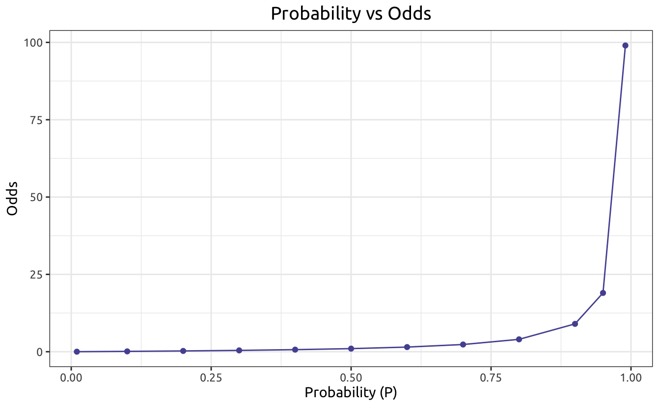
Imaging another scenario of drawing a ball from a packet, where there are 3 red balls and 2 blue balls. The probability of drawing a red ball is $3/5$, while the odds is $3/2$. This time, we have a larger difference, and the odds is even grater than one. In fact, the value of odds can be from 0 to positive infinity. Till now, we transformed from probability to odds.

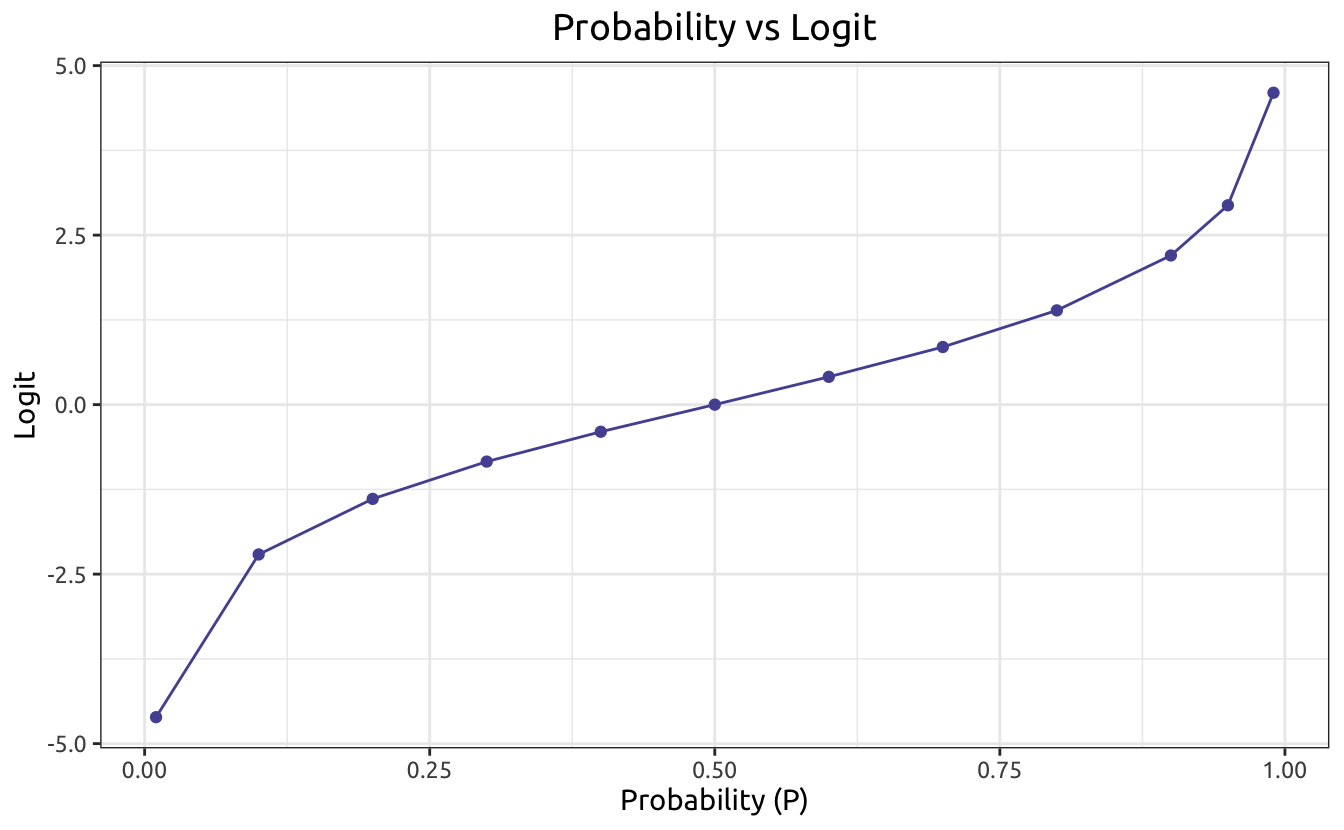
The next transformation is from odds to logit. This can be simply done by taking the log value of odds:

\[ \text{Logit} = \log(\text{Odds}) \]

Therefore, the full Logit Transformation is:

\[ \text{Probability} = P \rightarrow \text{Odds} = \frac{P}{1-P} \rightarrow \text{Logit} = \log(\text{Odds}) \]

To better explain the differences between these 3, I constructed a data frame and sketched 2 plots of P vs Odds and P vs Logit:

P	Odds	Logit
0.01	0.01	-4.61
0.10	0.11	-2.21
0.20	0.25	-1.39
0.30	0.43	-0.84
0.40	0.67	-0.40
0.50	1.00	0.00
0.60	1.50	0.41
0.70	2.33	0.85
0.80	4.00	1.39
0.90	9.00	2.20
0.95	19.00	2.94
0.99	99.00	4.60

A summary of the transformation:

Probability values range from $0$ to $1$.
Odds values range from $0$ to $+\infty$.
Logit values range from $-\infty$ to $+\infty$.

--- title: "The History of Logit" date: "May 20, 2024" categories: [Logit] format: html: code-fold: true code-tools: true --- ```{r} #| label: setup #| include: false library(tidyverse) library(kableExtra) library(here) ``` ## Useful Links | | | |-------------------|-----------------------------------------------------| | Research Paper | <a href="https://papers.tinbergen.nl/02119.pdf" class="btn btn-primary btn-sm" role="button"> The Origins of Logit Regression </a> | | Lecture Slides | <a href="https://hw.pingfanhu.com/emse_6035_hw/choice_modeling_slides/1_choice_modeling.pdf" class="btn btn-info btn-sm" role="button"> Intro to Choice Modeling </a> | | Online Article | <a href="https://zhuanlan.zhihu.com/p/27188729" class="btn btn-success btn-sm" role="button"> What is Logit (Chinese) </a> | ## Abstract This blog describes a brief history of the Logit Model. It starts from the famous Malthus population problem, and explains the necessity of transforming from probability to logit. ## The Malthus Population Problem ### 1. The Malthusian Growth Model In the biology class of my high school, I learned that the population will grow exponentially given unlimited resources and spaces. This is called the "Malthus Population Problem" and was give the name "J Curve", since the exponential Malthusian Model looks like the English letter J. The Malthusian Growth Function: $$ N_t = N_0 \cdot e^{rt} $$ Where: - $K$ (not in this equation but will be used later) stands for the carrying capacity, which is the maximum allowed population in the system. - $N_t$ stands for the population size at time of $t$, - $N_0$ stands for the initial population size, and - $r$ stands for the growth rate. The Malthusian Growth Model (CDF): ```{r} # Parameters K <- 10000 N_0 <- 100 r <- 1 # Calculation x <- seq(0, 10, length.out = 400) N_t_malthus <- N_0 * exp(r * x) data_malthus <- data.frame(Time = x, Population = N_t_malthus) # Plotting ggplot(data_malthus, aes(x = Time, y = Population)) + geom_line(color = "#5654A2") + labs(title = "Malthusian Growth Model", subtitle = expression( paste("Parameters: ", K, "=10000, ", N[0], "=100, ", r, "=1") ), x = "Time (t)", y = expression(paste("Population (", N[t], ")"))) + ylim(0, 10000) + theme_bw(base_family = 'Ubuntu') + theme(plot.subtitle = element_text(hjust = 0.5, size = 10), plot.title = element_text(hjust = 0.5, size = 14)) ``` In this model, we set a simple scenario of $K$ = 10,000, $N_0$ = 100, and $r$ = 1. It can be seen that the population grows so fast, that it reaches the cap while $t$ value is a little over 4. ### 2. The Logistic Growth Model However, this exponential model is unrealistic due to the scarcity of resources and spaces. A Belgian mathematician named Verhulst realized the cap of population growth. He used an S curve to explain this cap. This S curve is perhaps the first S-shaped curve that we could learn in our textbooks. Verhulst named this distribution "logistique", originated from a French word "logis", meaning "lodging" in English. However, we used the word "Logistic" instead for statistical analysis. This model is thus called the "Logistic Model", or "Logit Model". > The word "**logit**" is a portmanteau, coming from **logi**stic + uni**t**. The Logit Growth Function: $$ N_t = \frac{K}{1 + \left( \frac{K - N_0}{N_0} \right) e^{-rt}} $$ The Logit Growth Model (CDF): ```{r} # Calculation for Logistic Growth Model N_t_logit <- K / (1 + ((K - N_0) / N_0) * exp(-r * x)) data_logit <- data.frame(Time = x, Population = N_t_logit) # Plotting the Logistic Growth Model ggplot(data_logit, aes(x = Time, y = Population)) + geom_line(color = "#5654A2") + labs(title = "Logistic Growth Model", subtitle = expression( paste("Parameters: ", K, "=10000, ", N[0], "=100, ", r, "=1") ), x = "Time (t)", y = expression(paste("Population (", N[t], ")"))) + ylim(0, 10000) + theme_bw(base_family = 'Ubuntu') + theme(plot.subtitle = element_text(hjust = 0.5, size = 10), plot.title = element_text(hjust = 0.5, size = 14)) ``` This is the "S Curve" we've been seen in a lot of scenarios where there is a designed cap of population due to resource scarcity. There are also other S shaped curves. To avoid ambiguity, we use the term "Logit" instead. > The CDF of logit model is an S curve. With a visible diminishing of returns, it is a perfect model for human behavior studies for the purpose of generating a feasible marketing strategy. ## The Logit Model ### 1. Probability vs Logit The traditional way of defining the probability is to calculate the utility of choosing over the sum of utilities. The equation is written like this: $$ P_j = \frac{v_j}{v_j + v_k} $$ In this equation, the probability of choosing $j$ over $k$ is the utility of $j$ over the sum of utilities. In this model, utilities are normally distributed. An alternative way is to use the **Logit Model**, where we take the logarithm of the odds: $$ P_j = \frac{e^{v_j}}{e^{v_j} + e^{v_k}} $$ This is again the probability of choosing $j$ over $k$. To generalize the equation, the probability of choosing $j$ over all other alternatives is written as this: $$ P_j = \frac{e^{v_j}}{\sum_{k=1}^{J} e^{v_k}} $$ The logit model utilizes the Type 1 Extreme Value distribution, and requires independent errors (IIA). > IIA can be problematic when products are close substitutes. For example, in a DCM scenario, alternatives of Taxi, Red Bus, and Blue Bus are in fact 2 alternatives, since the Red Bus and the Blue Bus should be identical and only considered as one alternative. This is ignored by the IIA property. ### 2. Why Logit So, why using Logit Model? Why bother transforming the simple probability value into a somewhat non-intuitive value? An important reason is that the Logit Model does not have lower and upper limits. This can be better explained by the **Logit Transformation**: $$ \text{Probability} \rightarrow \text{Odds} \rightarrow \text{Logit} $$ In statistics, both probability and odds are used to describe the likelihood of an event occurring, but they have an important difference: 1. **Probability** refers to the ratio of the number of times an event A occurs to the total number of possible outcomes, while 2. **Odds** refers to the ratio of the probability of an event occurring to the probability of the event not occurring. The probability equation writes: $$ P(A) = \frac{\text{Number of Event A}}{\text{Total Number of Events}} $$ The probability $P$ is a real number between 0 and 1. $P = 0$ indicates that an event will definitely not occur, while $P = 1$ indicates that an event will definitely occur. In the case of rolling a die, the probability of rolling a 6 is: $$ P = \frac{1}{6} $$ The odds equation writes: $$ \text{Odds} = \frac{\text{Probability of event}}{\text{Probability of no event}} = \frac{P}{1 - P} $$ Continuing with the example of rolling a die, the probability of rolling a 6 is $P = \frac{1}{6}$, and the probability of rolling any other number is $1 - P = \frac{5}{6}$. According to the equation, the odds of rolling a 6 is: $$ \text{Odds} = \frac{1/6}{5/6} = \frac{1}{5} $$ Now you can see: The ratio of the probability of successfully rolling a 6 to that of not is 1:5. Like many other concepts in probability theory, the idea of odds originates from gambling. Suppose two people, A and B, bet on rolling a die; if A bets 1 dollar on rolling a 6, B would need to bet 5 dollars to ensure a fair game. $1/6$ and $1/5$ is not a big difference, but the point is to show that probability is *happening* vs *all*, while odds is *happening* vs *not happening*. Imaging another scenario of drawing a ball from a packet, where there are 3 red balls and 2 blue balls. The probability of drawing a red ball is $3/5$, while the odds is $3/2$. This time, we have a larger difference, and the odds is even grater than one. In fact, the value of odds can be *from 0 to positive infinity*. Till now, we transformed from **probability** to **odds**. The next transformation is from **odds** to **logit**. This can be simply done by taking the log value of odds: $$ \text{Logit} = \log(\text{Odds}) $$ Therefore, the full **Logit Transformation** is: $$ \text{Probability} = P \rightarrow \text{Odds} = \frac{P}{1-P} \rightarrow \text{Logit} = \log(\text{Odds}) $$ To better explain the differences between these 3, I constructed a data frame and sketched 2 plots of *P vs Odds* and *P vs Logit*: ::: {style="display: flex; flex-wrap: wrap; align-items: center;"} ::: {style="width: 30%;"} ```{r} #| echo: false # Define the probability values P <- c(0.01, 0.1, 0.2, 0.3, 0.4, 0.5, 0.6, 0.7, 0.8, 0.9, 0.95, 0.99) # Calculation Odds <- round(P / (1 - P), 2) Logit <- round(log(Odds), 2) # Data frame data_logit <- data.frame(P, Odds, Logit) data_logit %>% kable(escape = FALSE, align = c("c")) %>% column_spec(column = 1, width = '10em') %>% column_spec(column = 2, width = '10em') %>% column_spec(column = 3, width = '10em') %>% kable_styling(position = "center") ``` ::: ::: {style="width: 70%;"} ```{r} #| echo: false #| out-width: 90% # Plot P vs Odds ggplot(data_logit, aes(x = P, y = Odds)) + geom_point(color = "#5654A2") + geom_line(color = "#5654A2") + labs(title = "Probability vs Odds", x = "Probability (P)", y = "Odds") + theme_bw(base_family = 'Ubuntu') + theme(plot.title = element_text(hjust = 0.5, size = 14)) ``` ```{r} #| echo: false #| out-width: 90% # Plot P vs Logit ggplot(data_logit, aes(x = P, y = Logit)) + geom_point(color = "#5654A2") + geom_line(color = "#5654A2") + labs(title = "Probability vs Logit", x = "Probability (P)", y = "Logit") + theme_bw(base_family = 'Ubuntu') + theme(plot.title = element_text(hjust = 0.5, size = 14)) ``` ::: ::: A summary of the transformation: 1. **Probability** values range from $0$ to $1$. 2. **Odds** values range from $0$ to $+\infty$. 3. **Logit** values range from $-\infty$ to $+\infty$.